Basic Formulas in Excel
Excel has a variety of formulas and functions. If we want to insert a formula in Excel, then we need to get into the edit mode of the cell where we want to apply and then type equal (“=”) sign. This process activates all the functions or formulas of excel. There we can search for anything we want. We can use any basic operation here such as Sum, Average, Percentile, Vlookup, Mean, Etc. Suppose if we want to apply Sum function, then we need to select all the cells with the number here. And if you want to calculate Sum using basic Formulas, then we need to choose each cell followed by Plus (“+”) sign to find the Sum.
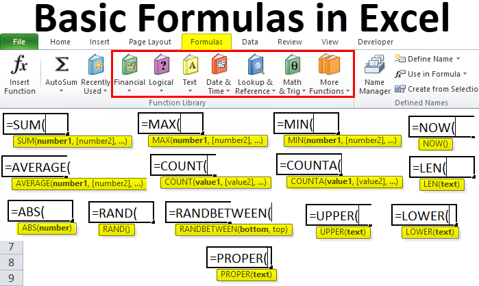
All the formulas in excel are located under the Formula tab in excel.
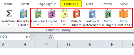
If you observe under Formulas tab we have many other formulas. According to the specialization each formula is located under its main tab. We have Financial, Logical, Text, Date & Time, Lookup & Reference, Math & Trig, and More Function. If you go through every section it has abundant formulas in it.
Going through all the formulas is not an easier task. In this article, I will concentrate only on the basic day to day excel formulas.
How to Use Basic Formulas in Excel?
Excel Basic Formulas is very simple and easy to use. Let’s understand the different Basic Formulas in Excel with some example.
Formula #1 – SUM Function
I don’t think there is anybody in the university who does not know summation of numbers. Be it an educated or uneducated adding numbers skill reached everybody. In order to make the process easy, Excel has a built-in function called SUM.
Look at the below data I have few numbers from the cell A2 to A5. I want to do the summation of a number in the cell A6.
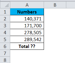
To get the total of the cells A2 to A5. I am going to apply the simple calculator method here. So the Result will be:
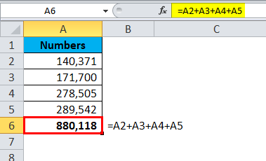
Firstly I have selected the first number cell A2 then I have mentioned the addition symbol +, then I have selected the second cell and again + sign and so on. This is as easy as you like.
The problem with this manual formula is, it will take a lot of time to apply in case of a huge number of cells. In the above example I had only 4 cells to add but what if there are 100 cells to add. It will be almost impossible to select one by one. That is why we have an inbuilt function called SUM function to deal with it.
SUM function requires many parameters it the each is selected independently. If the range of cells selected it requires only one argument.
Number 1 is the first parameter. This is enough if the range of cells selected or else we need to keep mentioning the cells individually.
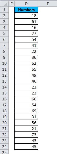
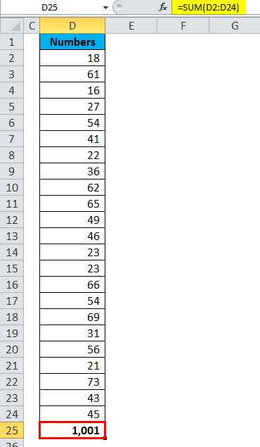
Look at the below example it has data for 23 cells.
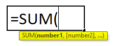
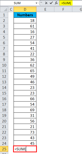
Now open the equal sign in the cell D25 and type SUM.
Select the range of cells by holding the shift key.
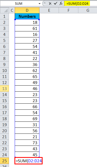
After selecting the range of cells to close the bracket and hit the enter button, it will give the summation for the numbers from D2 to D24.
Formula #2 – MAX & MIN Function
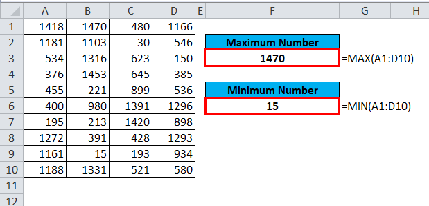
If you are working with numbers there are instances where you need to find the maximum number and the minimum number in the list. Look at the below data I have few numbers from A1 to D10.
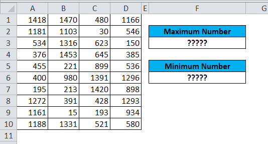
In the cell F3, I want to know the maximum number in the list and in the cell F6, I want to know the minimum number. To find maximum value we have MAX function and to find the minimum value we have MIN function.
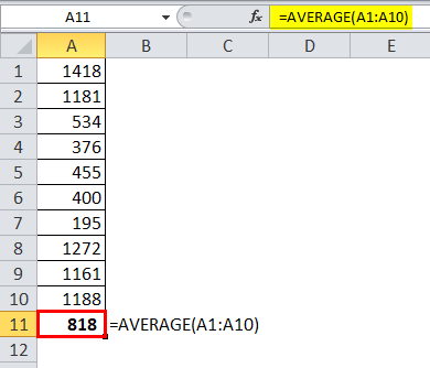
Formula #3 – AVERAGE Function
Finding the average of the list is easy in excel. Finding average value can be done by using an AVERAGE function. Look at the below data I have numbers from A1 to A10.
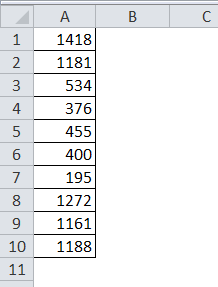
I am applying AVERAGE function in A11 cell. So the Result will be:
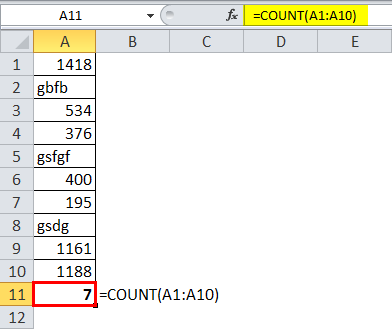
Formula #4 – COUNT Function
COUNT function will count the values in the supplied range. It will ignore text values in the range and count only numerical values.
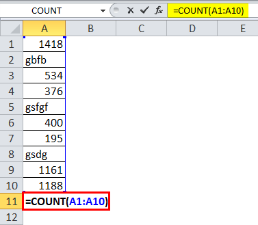
So the Result will be:
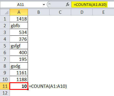
Formula #5 – COUNTA Function
COUNTA function counts all the things in the supplied range.
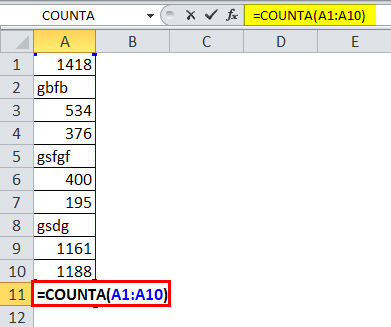
So the Result will be:
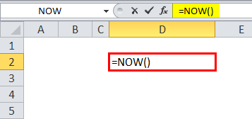
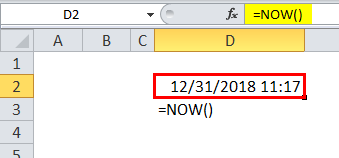
Formula #6 – NOW Function
If you want to insert the current date and time you can use NOW function to do the task for you.
So the Result will be:
Formula #7 – LEN Function
If you want to know how many characters are there in a cell, you can use the LEN function.
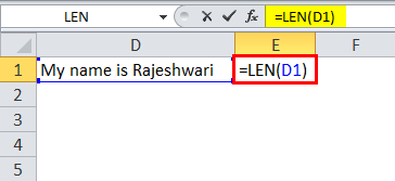
LEN function returns the length of the cell.
In the above image, I have applied the LEN function in the cell E1 to find how many characters are there in the cell D1. LEN function returns 21 as the result.
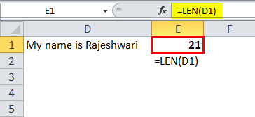
That means in the cell D1 total of 21 characters are there including space.
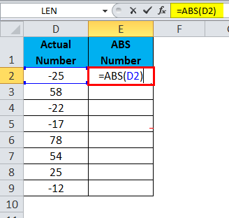
Formula #8 – ABS Function
If you want to convert all the negative numbers to positive numbers you can use ABS function. ABS means absolute.
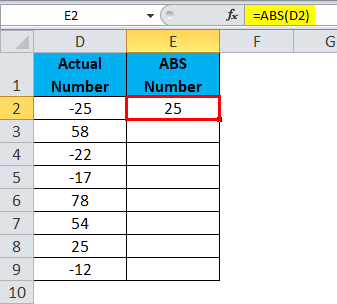
So the Result will be:
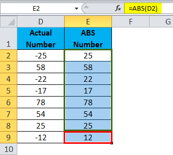
So the final output will occur by dragging cell E2.
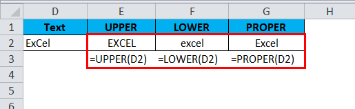
Formula #9 – UPPER, LOWER & PROPER Function
When you are dealing with the text values we care about their appearances. If we want to convert the text to UPPERCASE we can use an UPPER function, we want to convert the text to LOWERCASE we can use LOWER function and if we want to make the text proper appearance we can use the PROPER function.

No comments: